Introduction • PCGII

Intro

PCGII is an R package developed for Information-incorporated Gene Network Construction with FDR Control. PCGII stands for Partial Correlation Graphs with Information Incorporation.

To start using PCGII, prepare your gene expression data and your prior knowledge about gene-gene direct associations in the target network. Two methods were implemented in the package, PCGII for the case when you have prior knowledge and CLEVEL for the case when you do not have prior knowledge. You can select one of two methods to construct the gene network. Incorporating false information could lead to an inflation of the empirical FDR. As a result, we strongly recommend incorporating only high-confidence information in real data applications.

# Two ways to install PCGII
# Option 1
# install.packages("PCGII")
# Option 2
# devtools::install_github("HaoWang47/PCGII")
library(PCGII)
library(corpcor)
library(glmnet)
#> Loading required package: Matrix
#> Loaded glmnet 4.1-8
library(igraph)
#> 
#> Attaching package: 'igraph'
#> The following objects are masked from 'package:stats':
#> 
#>     decompose, spectrum
#> The following object is masked from 'package:base':
#> 
#>     union
library(Matrix)
library(mvtnorm)
library(tidyverse)
#> ── Attaching core tidyverse packages ──────────────────────── tidyverse 2.0.0 ──
#> ✔ dplyr     1.1.4     ✔ readr     2.1.5
#> ✔ forcats   1.0.0     ✔ stringr   1.5.1
#> ✔ ggplot2   3.4.4     ✔ tibble    3.2.1
#> ✔ lubridate 1.9.3     ✔ tidyr     1.3.1
#> ✔ purrr     1.0.2
#> ── Conflicts ────────────────────────────────────────── tidyverse_conflicts() ──
#> ✖ lubridate::%--%()      masks igraph::%--%()
#> ✖ dplyr::as_data_frame() masks tibble::as_data_frame(), igraph::as_data_frame()
#> ✖ purrr::compose()       masks igraph::compose()
#> ✖ tidyr::crossing()      masks igraph::crossing()
#> ✖ tidyr::expand()        masks Matrix::expand()
#> ✖ dplyr::filter()        masks stats::filter()
#> ✖ dplyr::lag()           masks stats::lag()
#> ✖ tidyr::pack()          masks Matrix::pack()
#> ✖ purrr::simplify()      masks igraph::simplify()
#> ✖ tidyr::unpack()        masks Matrix::unpack()
#> ℹ Use the conflicted package (<http://conflicted.r-lib.org/>) to force all conflicts to become errors
set.seed(010120000)

Simulate Network and Prepare Data

Three methods of generating a network structure were included in PCGII, including Scale Free Network Structure, Random Connection Network Structure, and Block Diagonal Network Structure. In this section, we will illustrate what are expected during data preparation. We will start with a network with 100 nodes.

## Simulate precision matrix as your true network structure
N_nodes = 100
N_samples = 30
Omega = make_sf_precision_mat(e = 1, p = N_nodes)

## Display the true network
nodenames = 1:N_nodes
links = which(lower.tri(Omega) & Omega!=0, arr.ind = TRUE)
dim(links) # display number of connections, two columns correspond to the connected nodes
#> [1] 99  2
my_net <- graph_from_data_frame(d=links, vertices=nodenames, directed=F) 
Ecolrs=c("gray50")
Vcolrs=c("gold")
plot(my_net, 
     edge.arrow.size=.5, 
     edge.color=Ecolrs,
     vertex.frame.color="#ffffff",
     vertex.label.color="black",
     vertex.size=3,
     layout=layout.auto(my_net)) 
#> Warning: `layout.auto()` was deprecated in igraph 2.0.0.
#> ℹ Please use `layout_nicely()` instead.
#> This warning is displayed once every 8 hours.
#> Call `lifecycle::last_lifecycle_warnings()` to see where this warning was
#> generated.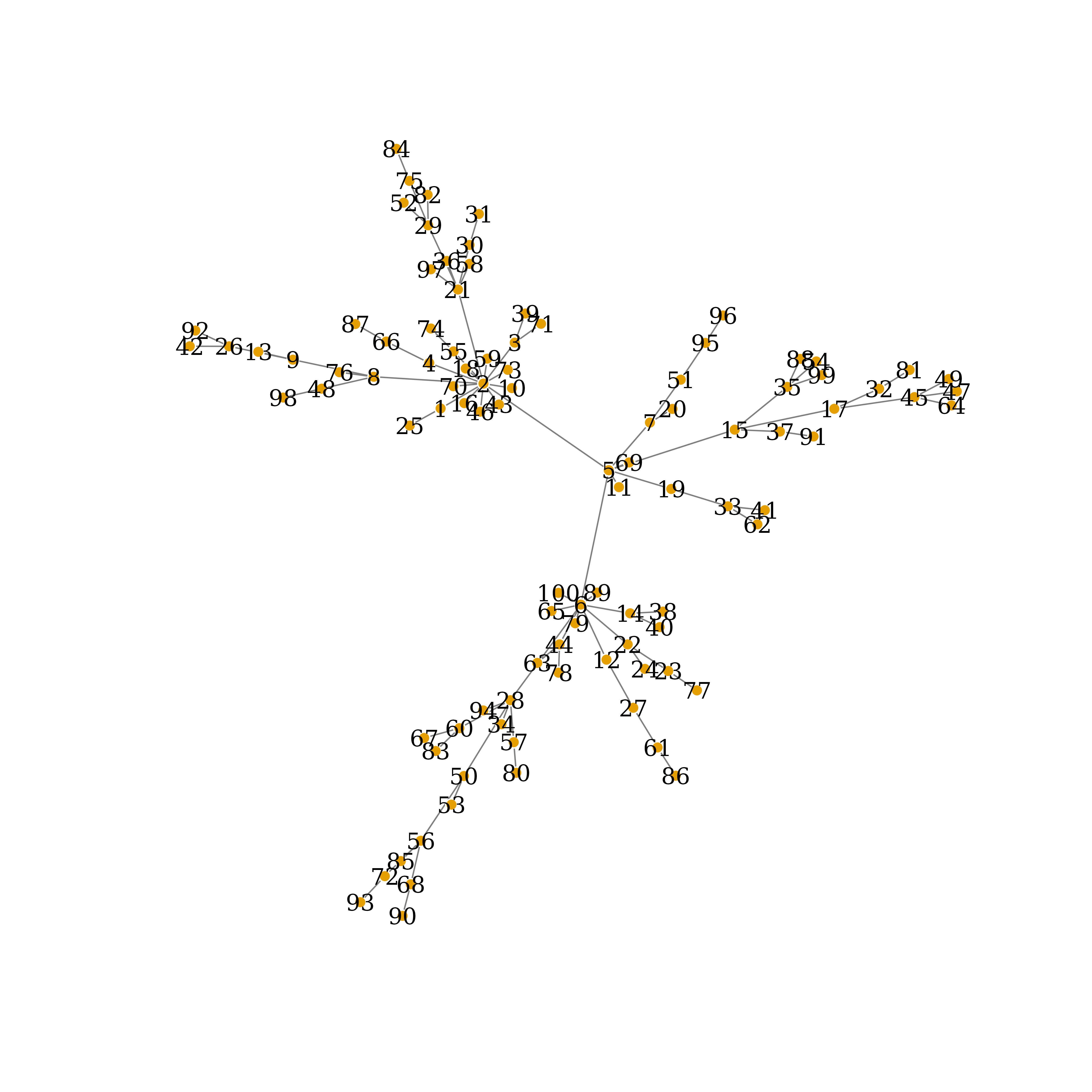

True Network Connections, auto-layout

plot(my_net, 
     edge.arrow.size=.5, 
     edge.color=Ecolrs,
     vertex.frame.color="#ffffff",
     vertex.label.color="black",
     vertex.size=3,
     layout=layout.circle(my_net))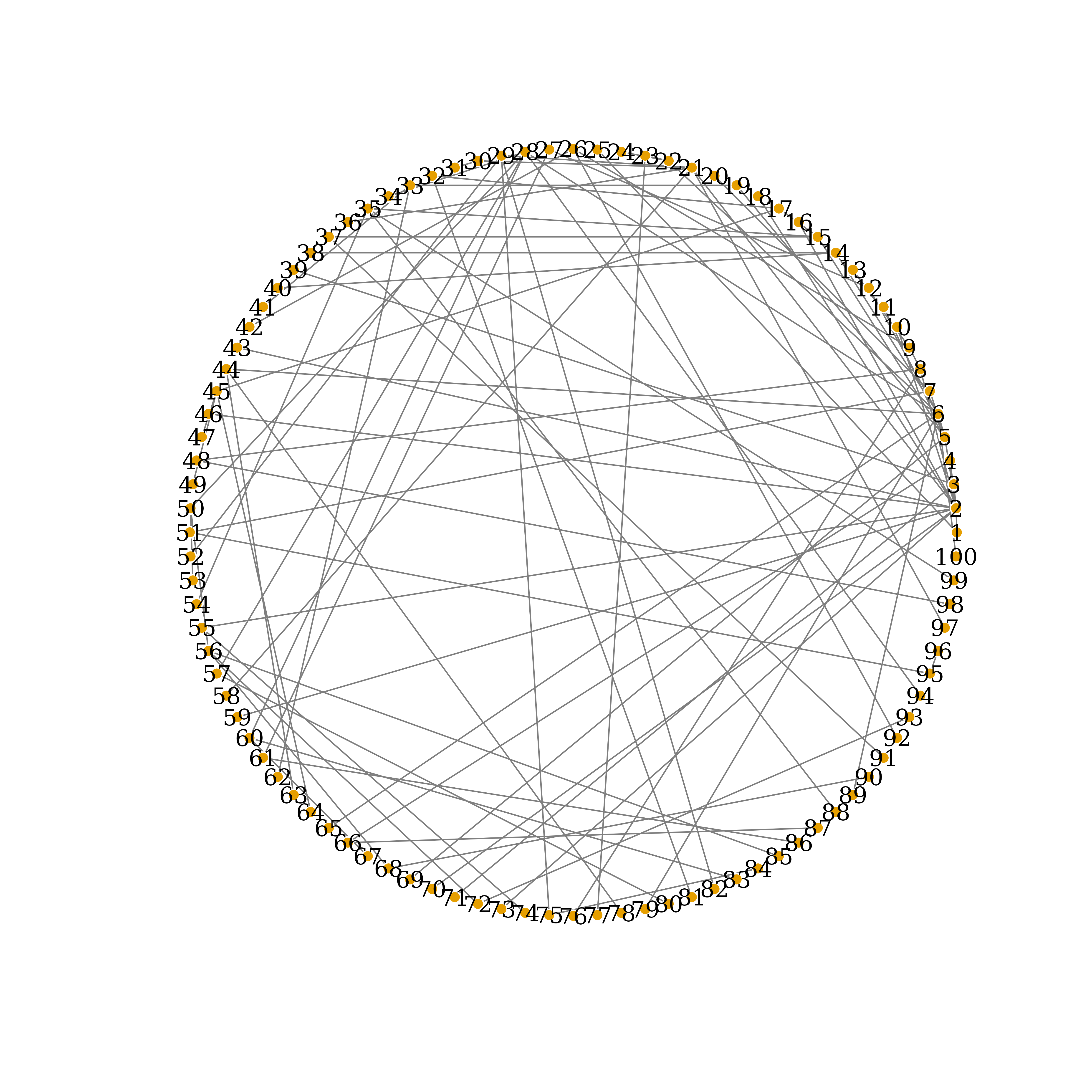

True Network Connections, circle-layout

## Simulate Normal data
Sigma = solve(Omega)
mu = exp(qnorm(seq(from = 0.01, to = 0.99, length.out = N_nodes), mean = 2, sd=1))
norm_data = mvtnorm::rmvnorm(n = N_samples, mean = mu, sigma = Sigma)
## Convert simulated normal data to expression count data
norm_data[norm_data<0] = 0
Exp_data = round(norm_data)
head(Exp_data[,1:10])
#>      [,1] [,2] [,3] [,4] [,5] [,6] [,7] [,8] [,9] [,10]
#> [1,]    0    0    0    3    1    3    1    2    3     2
#> [2,]    1    1    1    2    1    1    2    2    1     2
#> [3,]    0    1    1    1    3    1    0    3    1     4
#> [4,]    0    0    1    2    1    1    3    3    3     2
#> [5,]    3    0    2    4    0    2    1    4    0     0
#> [6,]    1    1    1    0    2    2    2    0    5     2

For illustration, we will randomly select a subset of true connections and use them as prior knowledge. It should be carefully considered if such prior connections are undirected (i.e. A-B OR A->B & B->A) in practice. Under the PCGII framework, it is recommended to use undirected connections as prior information.

prior_links = links[sample(1:nrow(links), .2*nrow(links)),]
types = rep(1, 99)
types[prior_links] = 2 # 1 for unknown true connections, 2 for known prior connections
undirected_prior_links = undirected_prior(prior_links)
prior_net = graph_from_data_frame(d=cbind(links,types), vertices=nodenames, directed=F) 
#> Warning in cbind(links, types): number of rows of result is not a multiple of
#> vector length (arg 2)
Ecolrs=c("grey90", "grey10") # dark grey shows known prior connections
E(prior_net)$color = Ecolrs[E(prior_net)$types]
Vcolrs=c("gold")
plot(prior_net, 
     edge.arrow.size=.5, 
     vertex.frame.color="#ffffff",
     vertex.label.color="black",
     vertex.size=3,
     layout=layout.circle(my_net))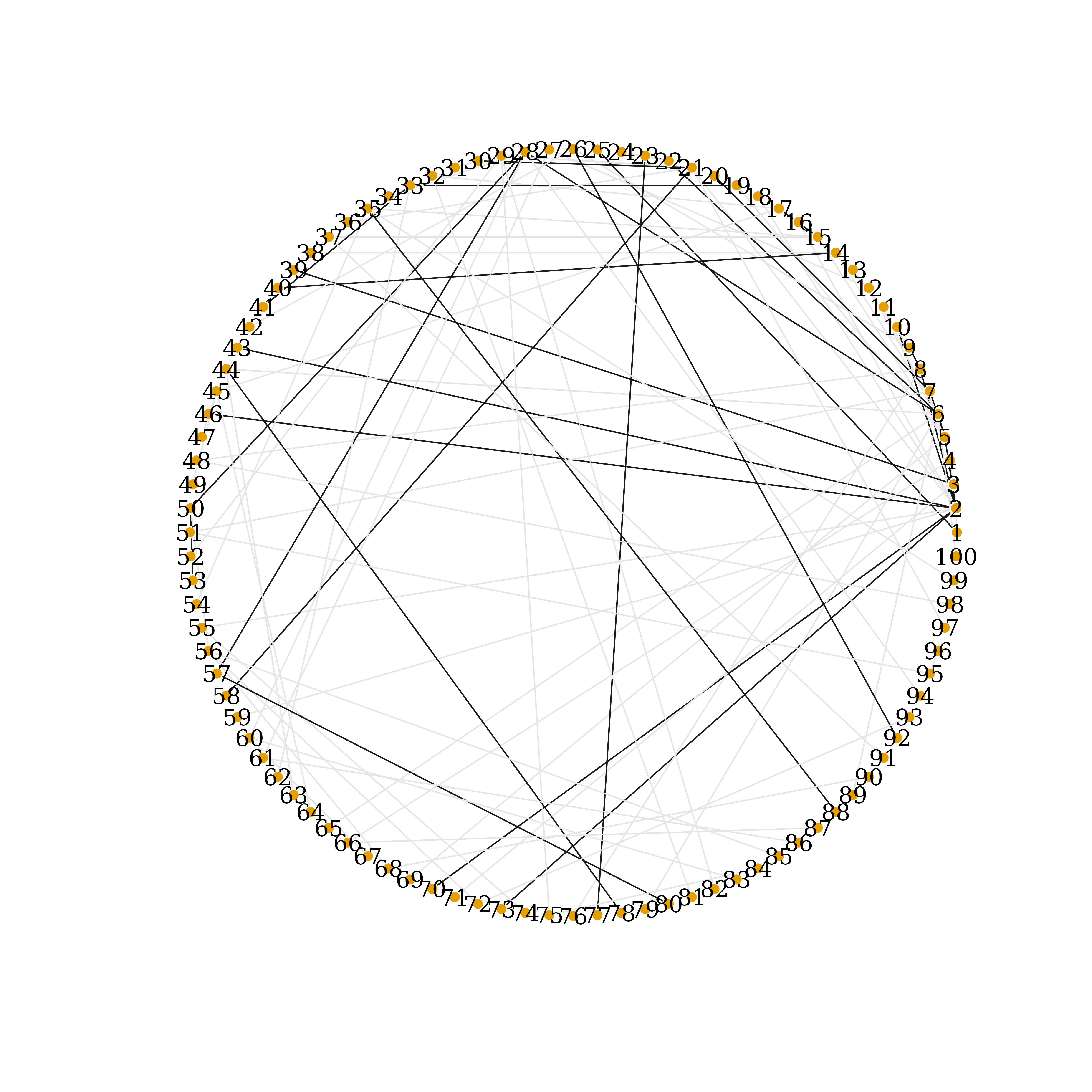

Prior Network Connections, circle-layout

Analyses with PCGII and CLEVEL

PCGII Inference

fixed_lamdba = sqrt(2*log(N_nodes/sqrt(N_samples))/N_samples)
PCGII.out = PCGII(df = Exp_data, prior = undirected_prior_links, lambda = fixed_lamdba)
PCGII.inf = inference(PCGII.out, alpha = .1)

Display significant connections detected by PCGII

PCGII_links = which(lower.tri(PCGII.inf) & PCGII.inf!=0, arr.ind = TRUE)
dim(PCGII_links) # display number of connections detected by PCGII
#> [1] 45  2
PCGII_net <- graph_from_data_frame(d=PCGII_links, vertices=nodenames, directed=F) 
Ecolrs=c("blue")
Vcolrs=c("gold")
plot(PCGII_net, 
     edge.arrow.size=.5, 
     edge.color=Ecolrs,
     vertex.frame.color="#ffffff",
     vertex.label.color="black",
     vertex.size=3,
     layout=layout.circle(PCGII_net))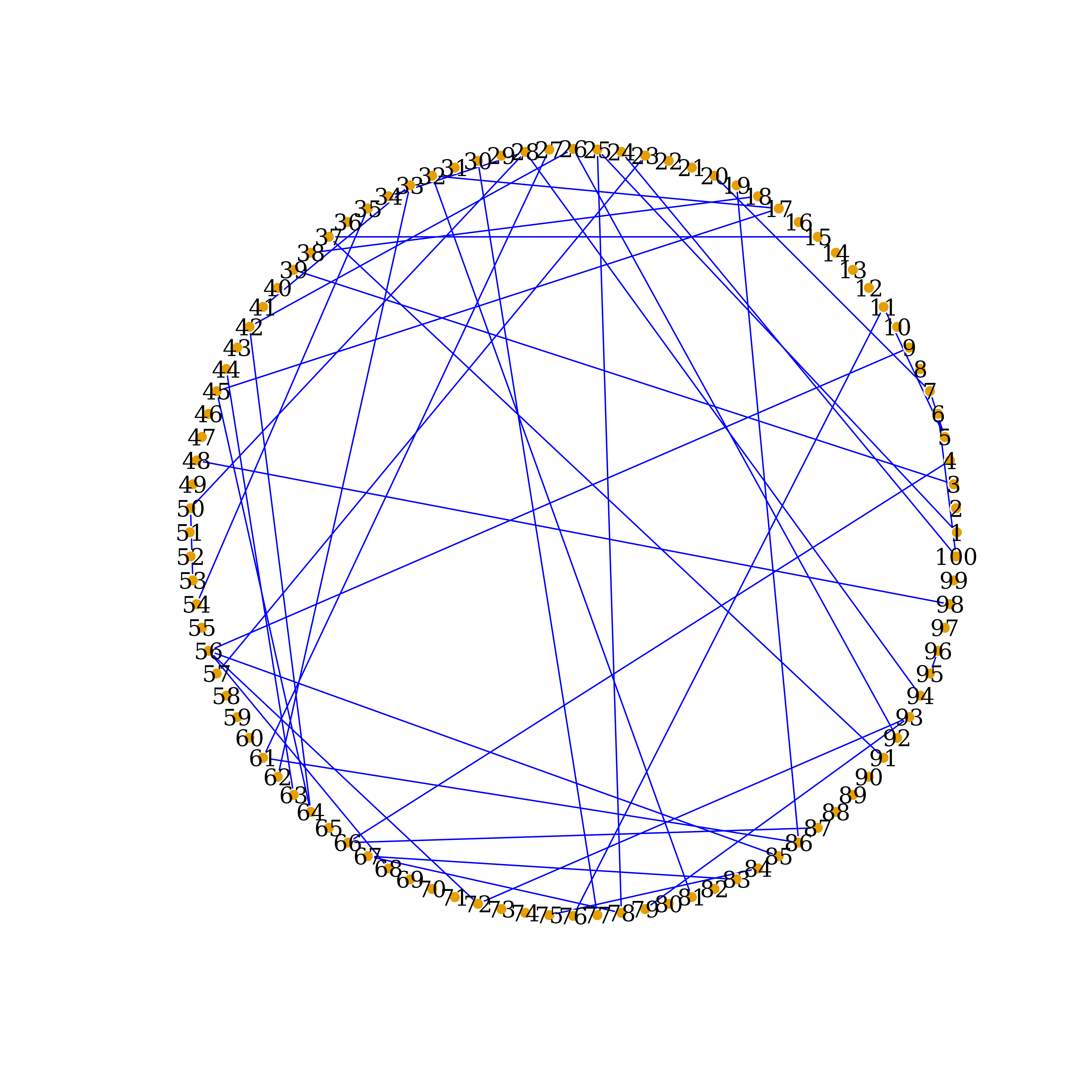

Network Recovered by PCGII, circle-layout

CLEVEL Inference

CLEVEL.out = clevel(df = Exp_data, lambda = fixed_lamdba)
CLEVEL.inf = inference(CLEVEL.out, alpha = .1)

Display significant connections detected by CLEVEL

CLEVEL_links = which(lower.tri(CLEVEL.inf) & CLEVEL.inf!=0, arr.ind = TRUE)
dim(CLEVEL_links) # display number of connections detected by PCGII
#> [1] 38  2
CLEVEL_net <- graph_from_data_frame(d=CLEVEL_links, vertices=nodenames, directed=F) 
Ecolrs=c("blue")
Vcolrs=c("gold")
plot(CLEVEL_net, 
     edge.arrow.size=.5, 
     edge.color=Ecolrs,
     vertex.frame.color="#ffffff",
     vertex.label.color="black",
     vertex.size=3,
     layout=layout.circle(CLEVEL_net))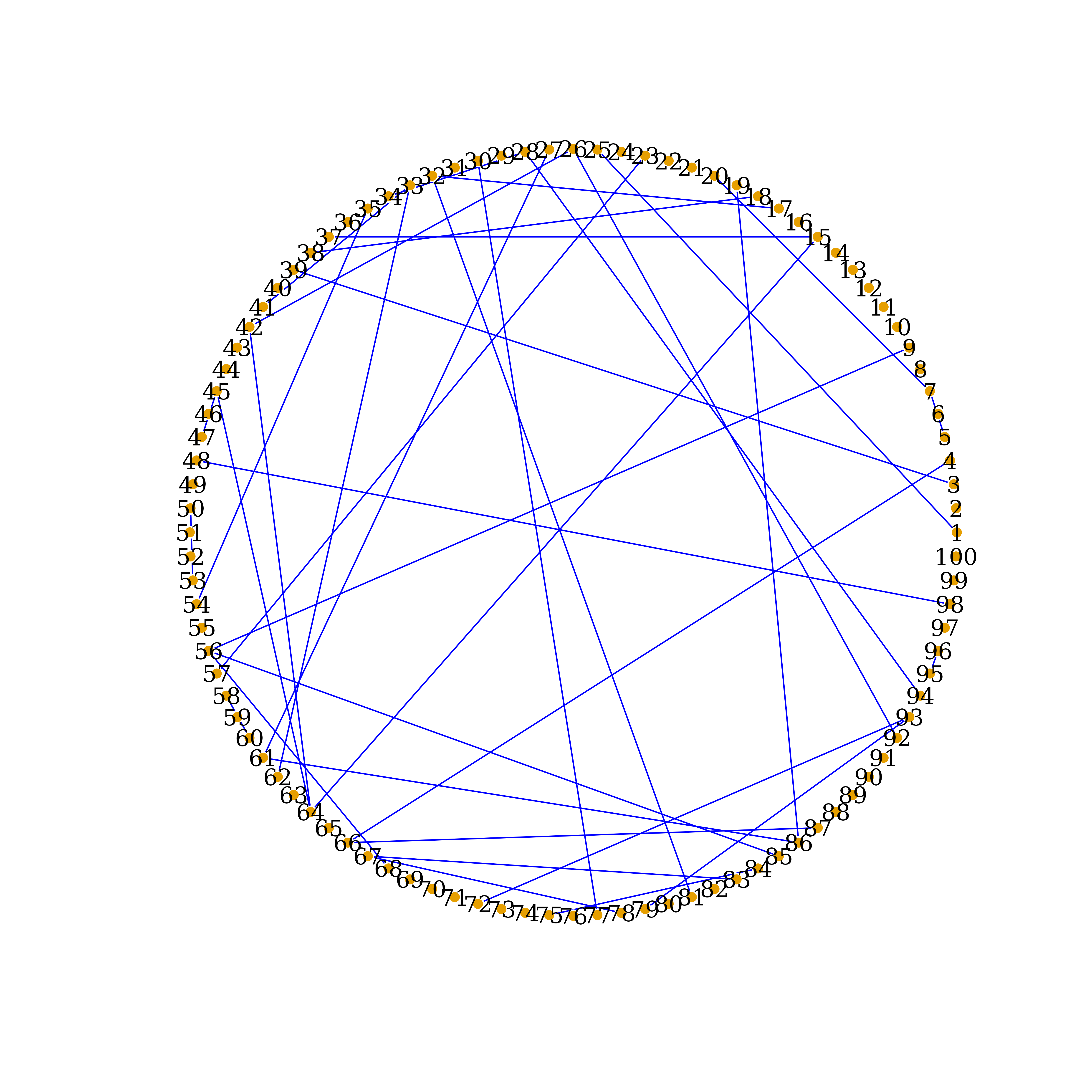

Network Recovered by CLEVEL, circle-layout